A couple weeks ago, Parse.ly published a blog post on why the media’s fixation on Trump is not supported by page view data. This post generated a good bit of criticism and controversy that I’d like to address here by untangling a couple of ideas and performing a more rigorous statistical analysis on the data.

One of the most contentious issues: How many articles should the media dedicate to each 2016 U.S. Presidential candidate? As with most should questions, there are some subjective issues at stake here, but with a couple of assumptions we can tease these issues out, leaving us with a well-defined and answerable question.

• Assumption 1: Above all else, the media wants to maximize page views.
• Assumption 2: It’s just as easy to write an article about any candidate.

We’re not arguing that these assumptions are correct–in reality, many factors inform the decision to write about a particular candidate, and many would argue (as we have before, and as we do below) that it is easier to write quick articles about Trump. Rather, in the spirit of a thought experiment, it’s informative to make these assumptions for now, reason about how the world would work if they were true, and then compare that world to reality. We’ll revisit these assumptions below.

Thought Experiment: What Would “The Bandit” Do?

Let’s say that journalists consult an algorithm that analyzes the performance of past articles and tells them which candidate to write about in their next article. This algorithm makes recommendations in such a way that, across the entire media, the number of page views is maximized. If writing more articles on a particular candidate results in diminishing returns, then this algorithm will recognize that, correct its course, and recommend other candidates accordingly.

Such algorithms exist and are known as multi-armed bandit algorithms. Multi-armed bandit algorithms come in many varieties and serve crucial roles in some of the web’s most profitable applications, such as Google’s ad serving systems.

Given the two assumptions above, we can rephrase our question regarding  which candidate journalists should write about as the following: If we were to feed a multi-armed bandit algorithm with industry-wide data on election news consumption, which candidate would it tell us to write about?

At Parse.ly, we have access to such information  and so we’ve actually run this thought experiment with real data. At the time this post was written, our election dataset includes more than 1.17 billion page views spread across 122,000 articles, collected from November 2, 2015 – May 29, 2016. You can interactively explore this data here (note that the data in our dataviz is updated every week, so you’ll see more data there than was used in this analysis).

With this data at hand, which of the many multi-armed bandit algorithms should we use? We choose to use a Bayesian technique called Thompson Sampling (also known as the Bayesian Bandit) for the following reasons:

• Thompson Sampling is known to be one of the best-performing bandit algorithms, while still being conceptually simple.
• The distribution of views per article has a long tail that many bandit algorithms will struggle with. Thompson sampling allows us to build up a Bayesian model that can take the heavy tail into account.
• Because this is a thought experiment, we want interpretable results. We don’t just want to know which candidate to write about next, we also want to clearly compare how articles on each candidate perform, with some estimate of how certain we are of that performance. By sampling the posterior of each candidate’s views per article distribution, we can nicely visualize which candidate’s articles are most popular.

Our Findings

While the results are summarized in the plot and table below, to understand what they mean you first need to understand the basics of Thompson Sampling, which is fortunately pretty simple.

We start by asking the question: What’s the average number of page views that an article on Donald Trump receives? However, rather than just calculating the average based on the sample of data that we have, we admit that our data is just a sample, so the average of this sample is likely somewhat inaccurate. We therefore construct a random model that’s most likely to have created the sample. This model is informed not only by the data we have on Donald Trump, but also by other prior information we have, such as:

• what the page view distribution for articles generally looks like;
• our best guess of the mean (or other relevant parameters) of that distribution; and
• how confident we are in that guess.

The great thing about having a model for the average page views (rather than just the average based on the sample we have) is that we can resample this model. Each time we resample the model, we get another guess at where the average lies. If the model is based on very little data and weak prior knowledge, then when you resample it many times it will give you wildly different estimates of where the average lies. However, if your model is fit on enough data, then its estimates of the mean will cluster tightly around a narrow range of values.

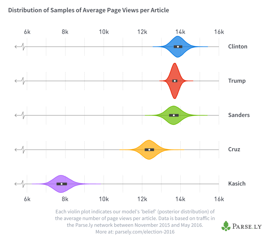
We built the same kind of model for each candidate, based on that candidate’s data. The following plot indicates where the average number of page views for each candidate is most likely to lie:

Each of the “violins” in this plot represents the probability density of a candidate’s average page views. In other words, we’re not sure exactly what the average number of page views is for each candidate, but the taller a violin is at any point, the more likely it is that the true average page views is located there. The white dots show the median of our samples, and the thick black bar represents the interquartile range.

Notice how Trump’s violin is taller and narrower than the others—this is because journalists wrote many more articles on him than on any other candidate, and so his model was based on more data. It’s therefore more confident about the average number of views that each Trump article receives.

With this visualization in place, it’s easy to explain how Thompson Sampling works. When you ask the algorithm for a recommendation, it samples each candidate’s model once, and then recommends you write an article on the candidate whose sample had the highest value. Once you actually write the article and observe how many clicks it receives, you need to update your probability distributions with that information. That’s basically all there is to Thompson Sampling. At its core, it selects a topic in proportion to how confident it is that the topic is the best.

Using the distributions displayed in the violin plots above, I can simulate what would happen if 100,000 journalists came along and asked our bandit algorithm which candidate to write on. The following table displays how many times the bandit would recommend each candidate.

Clinton		Sanders		Trump		Cruz		Kasich
52,962		25,450		21,579		9		0

These results suggest that, given readers’ long-term interest in each candidate, and the two assumptions we made above, right now the media should write 53 percent of its articles on Clinton, 25 percent of its articles on Sanders, and 22  percent  of its articles on Trump.

Note that this is not the same thing as saying that the data shows the media should have written 53 percent of its articles on Clinton over the last seven months. Bandit algorithms can only tell you what you should do right now, given your previous data.

Once you carry out a bandit’s suggested action, you need to update it with the result (i.e., the number of page views the article you just wrote received), and then the bandit can correct its course. So it could be that if the media actually started to write 53 percent of its articles on Clinton (rather than Trump), then the popularity of those articles would decrease, and the bandit would start suggesting that journalists write more on other candidates.

What About a More Timely, Useful Bandit?

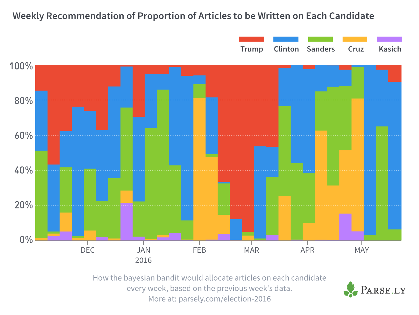
The bandit I constructed in the last section wouldn’t actually be all that useful for journalists in practice because it gives equal weight to all data from the last seven months, whereas readers’ interests change week by week as new stories unfold. So instead of creating one bandit based on the data from the last seven months, let’s create a separate one for each week’s worth of data that only includes articles written that week. We can then sample each week’s models like we did to create the table above, which gives us the proportion of articles that our bandit would recommend to write on each candidate, every week:

As we look at the chart above across time (left to right), the fluctuating vertical widths of the colors indicate that readers’ interests change rapidly. Trump receives the longest stretch being highly recommended by the bandit from mid-February to mid-March, but even this lasts only four weeks, and in one of those the bandit recommends writing slightly more on Clinton. Most weeks, the bandit recommends writing more on other candidates as a whole than on Trump, which the media hasn’t in fact done.

Conclusions: Comparing Our Thought Experiment to Reality

Let’s summarize what we’ve discovered in this thought experiment. We started with the subjective question ‘how much attention should the media give to each candidate’ and then made two assumptions.

• Assumption 1: Above all else, the media wants to maximize page views.
• Assumption 2: It’s just as easy to write an article about any candidate.

Given these assumptions, I claimed that a multi-armed bandit algorithm can objectively answer this question, and gave a high-level overview of how such an algorithm works. I then actually ran such an algorithm over real historical data in two different ways: first over all data we’ve collected since last November, and then over one week of data at a time.  The results of the former show that, given reader’s long-term interest, the media should currently be writing much more about Clinton, and much less about Trump. The results of the latter, week-by-week analysis, indicate that readers’ interests fluctuate wildly but are certainly not dominated by Trump.

Now let’s step out of the thought experiment entirely and admit that neither assumption is correct. What can we learn?

Assumption 1 claimed that journalists and editors produce content only to drive revenue through page views. In reality, many who pursue careers in media are primarily motivated by factors other than money, such as the desire to tell compelling stories; reveal unexpected truths; or, in the case of political coverage, to fulfill the important role that the media plays in creating an enlightened electorate. It’s hard to see how any of these motivations would lead the media to provide such lopsided coverage of Trump.

When the media has self-reflected on this topic, it has often shrugged its shoulders, admitted that such coverage contradicts its non-monetary motivations, and assumed that this lopsided coverage is due to the fact that articles on Trump produce more revenue. However, we have here shown that if the media really were primarily motivated by profit, then they would start writing many more articles on Clinton somewhat more on Sanders, and far fewer on Trump.

So why does the media write so much on Trump, given that it’s both counter to many journalists’ non-monetary ideals and irrational from the perspective of revenue-generation? Can we just conclude that the media’s irrational? Well, let’s not forget Assumption 2, which never seemed very plausible: it’s just as easy to write an article on any candidate. As we mentioned in our previous post:

In the midst of today’s 24-7 news cycle, most journalists … often find themselves choosing topics that are convenient to write about. Imagine you’re a journalist in front of a blank screen, thinking about your next story, and faced with intense pressure to pump out content. There may be no clear breaking news on Clinton, Sanders, Cruz, or Kasich — so writing about these candidates may require you to conduct research or reach out to voters. On the other hand, your Twitter feed is full of the ‘events’ that Trump so routinely creates and which feed personality-driven celebrity journalism: politically incorrect comments, bogus claims, and far-fetched promises.

In fact, one could argue that it’s not only more convenient to write about Trump, but that it’s more profitable. If you look at the problem from a return-on-investment perspective, you might argue along the following lines: it’s so much easier to write on Trump that I could write ten articles on him or five on other candidates. Even though Trump articles receive fewer page views per article, the difference is small enough that it still makes sense to just write on Trump, because I’ll end up with more page views overall.

The results of the thought experiment above lead me to believe that it’s exactly this line of thought that drives the media to write more articles on Trump than all other candidates combined. At the end of this investigation, we’re left wondering whether it’s really easier to write articles on Trump, or that’s just an attitude adopted by many journalists. After all, at any moment in time there are dozens of possible topics one could write about any candidate, and how “hard” it is to write about any of these topics depends largely on the creativity and resourcefulness of journalists, themselves.

Source code and data

I encourage you to inspect and run the python code that I used in the experiment above.  You  can find the instructions, code, and data you’ll need to replicate my results here.

Appendix: Methodology

In this appendix, I’ll describe the main decisions we made in implementing the models described above, but I won’t go over how Thompson Sampling works in detail because it’s a topic that has been well covered elsewhere. For an accessible introduction to Thompson Sampling, see this section of the book Bayesian Methods for Hackers; for a more concise definition of Thompson Sampling along with empirical results, see this paper.

Determining the best page view distribution

The model we used here assumes that the number of views an article receives is a random variable drawn from a lognormal distribution. This is the single most important modeling decision we made, so it’s worth devoting some words here to explaining why we chose the lognormal distribution.

A quick look at the data indicates that the distribution in question is fat tailed–in other words, the number of page views that an article receives varies wildly, with a small proportion of articles accounting for a large proportion of page views. For example, if we rank articles by the number page views they receive, the top two percent received about 50 percent of all page views.

While I was in grad school, it was popular and exciting to assume that fat-tailed distributions were best described as exotic power-law distributions. Luckily, the backlash to this fad has led the statistics community to create a useful python library called power-law. This library makes it easier to judge whether it’s appropriate to call your distribution a power-law distribution by calculating goodness of fit and creating the appropriate plots that enable visual inspection. The library checks to see whether the much less exotic lognormal distribution might be a better fit.

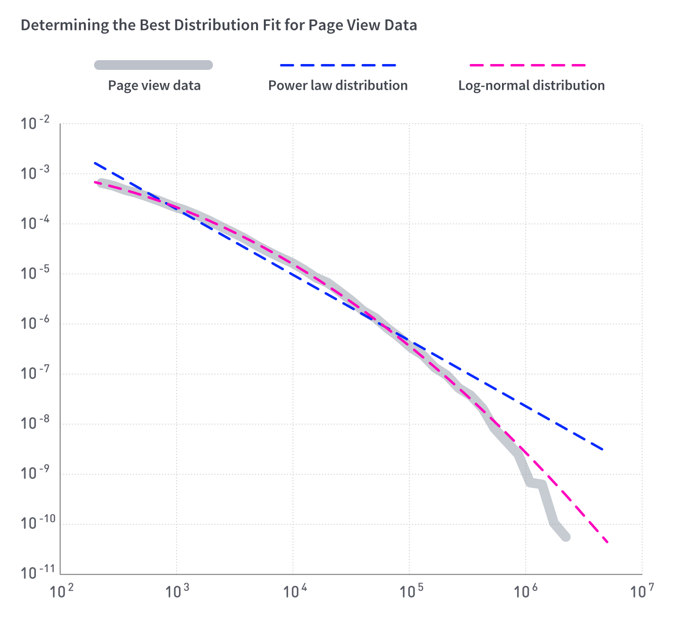
As is evident in the plot below, the lognormal distribution fits better than the power-law distribution:

The parameters of each distribution were fit by the power-law library by calling the running the fit function with the following parameters:

fit = powerlaw.Fit(data, discrete=True, xmin=200, xmax=data.max())

Note that I set the xmin parameter to equal 200 page views–this means that the power-law library ignores all data points that have fewer than 200 views. Why do I ignore these data points? In short, the lognormal distribution fits better than the power law distribution regardless of the value of the xmin parameter, but a lognormal distribution fit on data points >= 200 fit much better than a distribution fit on all of the data.

The longer explanation is that it appears that articles that receive fewer than 200 page views may obey different scaling laws than articles that receive more page views. It could be, for example, that articles in this regime include unfinished drafts of articles tracked by our system, unpopular articles written by corporate public relations teams, automated reports, or articles written by obscure and unpromoted bloggers (rather than professional journalists who receive the support of their publishers).

Because we’re most interested in providing advice to professional journalists, we exclude articles that receive fewer than 200 hits from the analysis presented here. If you’re a journalist and know your article will have more than 200 page views, even if it’s a flop, then this modeling decision allows us to fit a more accurate model by removing just the 0.16 percent of the total page views from the dataset that come from the least popular articles (note that this also removes 44 percent of the articles from the dataset).

Sampling the posterior

Given that we’ve settled on using a lognormal distribution, how do we actually sample the posterior, which allows us to estimate where the mean number of pageviews lies for each candidate? We need a function that takes in our prior beliefs about the page view distribution, combines it with the data we collected, and returns a sample. We found such a function implemented in python in this excellent blog post from Sergey Feldman, which, in turn, is based on the method outlined in Gelman et al’s Bayesian Data Analysis.