Lucene: The Good Parts

Before MongoDB, before Cassandra, before “NoSQL”, there was Lucene.

Did you know that Doug Cutting wrote the first versions of Lucene in 1999? To put things in context, this was around the time Google was more a research project than an actual trusted application. Google’s proof-of-concept search engine was still a sprawling set of desktop computers in Stanford’s research labs.

I worked on my first Lucene project around 2005. It was a document management system. It didn’t have any real issues of scale — it was a web application meant to be run on-premise and to provide a view of data that could safely fit in a hard drive or NAS.

But, even though the total dataset measured in the hundreds of gigabytes, searching through all the data efficiently was still a challenge. SQL was not then, and is still not now, a very good blob or document storage system. Yet, there seemed to be no alternative to SQL for durability, short of relying directly upon the filesystem. To boot, the primary use case of the application I was working on was actually document search. People needed to find things. All SQL databases stink at unstructured search, so that’s why I started researching Lucene.

Lucene was a Java library you had to learn, and then manually integrate into your app. Thankfully, this wasn’t as hopeless as it sounds now.

Among Java projects, Lucene was exceptionally well-documented. Further, Lucene in Action had been published in 2004, and the book went into a lot of depth on how the whole library worked. I remember purchasing my copy and devouring the book in a weekend. I remember thinking, at the time, that it was probably one of the best technical books I had read — not just about Lucene, but in general!

Lucene in Action is now available in a 2nd Edition that updates it for Lucene 3.0 — though, it could probably use yet another update, as Lucene 5.0 was recently released!

A couple of things struck me about Lucene after my first project working with it. First, Lucene approaches problems of data exploration from the vantage point of “information retrieval”, not from the vantage point of “database management theory”. This meant Lucene was less concerned with things like MVCC, ACID, and 3-NF, and was instead concerned with much more practical concerns, like how to build a fast and humane interface for unstructured data.

Lucene’s creator pondered: How do we support queries that normal users will actually type? How do we rapidly search all the data we have, in one fell swoop? How do we order the results when there is more than one likely match? How do we summarize the full result set, even if we only have enough space to display part of the result set?

At the time, Solr and Elasticsearch didn’t yet exist. Solr would be released in one year by the team at CNET. With that release would come a very important application of Lucene: faceted search. Elasticsearch would take another 5 years to be released. With its recent releases, it has brought another important application of Lucene to the world: aggregations. Over the last decade, the Solr and Elasticsearch packages have brought Lucene to a much wider community. Solr and Elasticsearch are now being considered alongside data stores like MongoDB and Cassandra, and people are genuinely confused by the differences.

Google Trends shows declining search interest in Lucene, even as Solr and Elasticsearch interest rises. How odd — Lucene is what makes it all work!

So, I thought it might be fun to go back to basics. What’s so good about Lucene? How does it work under the hood? And why does that give a system like Elasticsearch a leg up on a system like Cassandra in certain applications? Finally, what can we learn from Lucene even if we don’t care about full text search?

Jargon terms

So, let’s start with a de-jargoning exercise. Here are some terms you see thrown around in the Lucene and Information Retrieval communities which are not nearly as common in the SQL and database communities. Lucene even re-defines the term “term” — so, please, pay attention!

document: a record; the unit of search; the thing returned as search results (“not a row”)
field: a typed slot in a document for storing and indexing values (“not a column”)
index: a collection of documents, typically with the same schema (“not a table”)
corpus: the entire set of documents in an index
inverted index: internal data structure that maps terms to documents by ID
term: value extracted from source document, used for building the inverted index
vocabulary: the full set of distinct terms in a corpus
uninverted index: aka “field data”, array of all field values per field, in document order
doc values: alternative way of storing the uninverted index on-disk (Lucene-specific)

OK, that gets some jargon out of the way.

Inverting our corpus

Let’s start with a simple corpus of: two documents, doc1 and doc2, both contain the field “tag”, type “string”, with the text “big data”. There is also doc3, same structure, but its tag contains the text “small data”.

With this small corpus, how can we find things?

Instead of storing:

doc1={"tag": "big data"}
doc2={"tag": "big data"}
doc3={"tag": "small data"}

We can store the “inverted index”. What’s that?

big=[doc1,doc2]
data=[doc1,doc2,doc3]
small=[doc3]

Ah, so it’s not an index of documents to terms, it’s an index of terms to documents. Clever. If we organize the data this way, we can find documents by value more quickly. When I search for “big”, I get back doc1 and doc2. If I search for “small”, I get back doc3. If I search for “data”, I get back all documents. This is basically the core data structure in Lucene and in search in general. Yay for the inverted index!

Lucene spreads its index across several on-disk files, each format purpose-built for a specific use case. These files are organized into logical “segments” that represents subsets of documents across the corpus.

Not in my vocabulary

In the above documents, I have 3 “terms”, and the assumption is that I generated them by doing basic whitespace tokenization. So, my original corpus had the field values ["big data", "small data"], but my generated terms are ["big", "small", "data"].

This already suggests something interesting about terms. If information is repeated in your field values, it will be compressed by pulling out the terms.

By the way, if I were to leave those fields unanalyzed, I’d have two terms: they’d be “big data” and “small data”. If I decide not to analyze a field, but I decide to store it (in Lucene “stored” field or in Elasticsearch “_source” field), then I am essentially storing the data twice. Once, in the inverted index, and once in the “field storage” (wherever that is), as well.

Terms are interesting when you have data that repeats frequently among your documents. In this small example, the term “data” is repeated in both documents, but only requires one entry in the inverted index. Imagine the same kind of corpus as above, but where you have 1,000 total documents, half tagged with “big data” and half tagged with “small data”. In this case you might have:

data=[1,2,3,...,1000]
big=[1,3,5,7,9,...,999]
small=[2,4,6,8,...,1000]

Here, the inverted index stores one entry for “data”, even though data appears in 1,000 documents. It stores one entry for “big”, even though it occurs in 500 documents. Likewise for “small”.

Big data concordance

You might do a quick back-of-the-envelope calculation at how much more efficient it is to store an inverted index of this data than to store a normal document-to-term index.

Storing the document IDs repeatedly isn’t free, but it’s certainly cheaper than storing the whole document repeatedly. The vocabulary of a large data set will tend to be much smaller than the record storage of that same data set, and we can take advantage of this at scale.

By the way, this is a pretty ancient technique of mining data. The first complete vocabulary of a complex text was constructed in the year 1262, by 500 very patient monks. The document in question was, of course, the Bible, and the vocabulary was called a concordance. How does that proverb go? “There is nothing new under the sun.”

An example biblical concordance, this one a bit more modern than the one the monks may have worked on.

Discretely numerical

Have a lot of text data you need to make sense of? You clearly have a “search” problem. Have a lot of numeric data you need to make sense of? Well, now, of course, you have an “analytics” problem. Different problem, right?

Well, maybe. The benefits of the inverted index, terms, and vocabularies apply equally well to numeric data. It just requires some lateral thinking to get there.

The reason fields need to have types is because the way we index field values into terms can dramatically affect how we can query those fields. Text is not the only thing that can be broken into terms — numeric and date field values can, as well. This is a bit mind-bending, as terms feel like a text-only concept.

Here’s a snippet from Lucene in Action on the topic: “If you indexed your field with NumericField, you can efficiently search a particular range for that field using NumericRangeQuery. Under the hood, Lucene translates the requested range into the equivalent set of brackets in the indexed trie structure.”

The equivalent set of brackets in the indexed trie structure? Sounds fancy. To start with, what trie structure are we talking about?

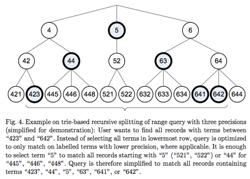
An example trie data structure storing numeric data.

Here’s an example. So, let’s suppose I add a new field to my documents called “views”. It is a numeric field that contains the number of views each document received on some website. The section above explained how we might find documents that have certain ranges of views, e.g. views between 50 and 100.

If I convert the “views” field into terms, I’ll have something that looks like this, perhaps:

49=[doc31]
50=[doc40,doc41]
51=[doc53]
...

This isn’t very helpful. To query for a range of views from 50 to 100, I’d have to construct 50-part query, one for each discrete term:

50 OR 51 OR 52 ... OR 100

The solution, as mentioned above, is a “trie structure of brackets”. Lucene will automatically generate terms that look more like this:

49=[doc31]
50=[doc40,doc41]
50x75=[doc40,doc41,doc53,doc78,doc99,...]
51=[doc53]
...

Notice that 50x75 is a special term that encompasses a bracket of 25 discrete values, and thus points to a lot of documents. This allows for smaller queries to cover ranges, and a quicker retrieval of documents over large ranges. The idea is to reduce the discrete numeric data set to a number of lumpier “term ranges”. So now, we might be able to cover our 50-100 range with a query like this:

50x75 OR 76x99 OR 100

The key thing is to select these term ranges automatically — and Lucene has an algorithm for that which ensures that there are enough terms to cover all ranges with good average speed.

Pretty magical, huh? Here’s the other clever thing: because numeric values can be converted to term ranges, this same magic works on dates, as well. The dates are converted to numbers, the numbers are then converted into term ranges. Thus, even though you might be searching through 1 million “minutes” of data, you would only be searching through a few hundred “minute ranges” in the inverted index. We could even call these “minute ranges”, well, “days”!

If you need a more visual explanation of numeric range queries, check out this slideshow.

The UNIX philosophy introduced the abstraction that “everything is a file”, and it certainly required some lateral thinking to make devices like printers and network sockets feel like files. The Lucene philosophy equivalent is, “everything is a term”. Numbers, dates, text, identifiers, all can be mapped to behave like text terms, with all the same benefits.

Just uninvert what you’ve inverted

But, we’d still like to do something with the values within this field. For example, we might like to aggregate up the total views across all of our documents, what in SQL might be a sum() aggregate. We might also want to find the document with the most views, that is, to sort our documents by their number of views.

To do this, our inverted index is no help. We might have values ranging from 0 to 100 million in there, with each discrete value (or synthetic range) pointing to the right document IDs. We don’t want to find the documents with certain values; we want to instead calculate summaries (aka “analytics”) over our corpus or some subset thereof.

A new problem demands another lateral thinking solution. Why don’t we uninvert the inverted index? Huh?

In other words, why don’t we store, per field, an array of field values, in document order? An index, not of terms to document IDs, but an index of field values that we know (by their order) correspond to specific documents.

views=[1,1000,5000,1000000,200,...]

When we need to do calculations across the whole corpus, we can slurp this array into memory (and, perhaps, keep it there for later). We can then run calculations as fast as computationally possible. If you need to execute a sum() on some subset of this array, we can use another trick, Bitsets, for filtering down the array as we go.

The quickest bit

A quick detour. I first heard of Bitsets in one of my favorite programming books, an oldie but goodie passed down to me by my Dad. It’s called Programming Pearls.

Its first problem, entitled “Cracking the Oyster”, involves solving a specific file sorting problem by representing the lines of the file as an array of bits, where each bit represents one of the possible line values. As described in that chapter, the Bitset is “a dense set over a finite domain when each element occurs at most once and no other data is associated with the element”. The author observes that programmers should seek cases where “reducing a program’s space requirements also reduces its run time,” something he refers to as “mutual improvement”. Properly applying a Bitset to a sorting problem is one such example.

Admit it — part of the reason you went into software is because you thought working in binary and doing bit arithmetic was pretty cool. After all, there are only 10 kinds of people in this world, those who understand binary, and those who don’t.

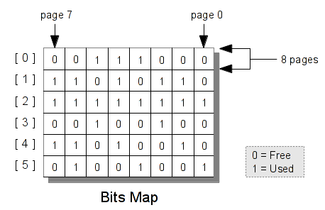
Let’s return to our uninverted index. Let’s say that you want to only sum views from documents that match a specific author. In this case, the full array of views will be compared against a Bitset that might look as follows:

views=[1,1000,5000,1000000,200,...]
specific_author=[0,1,0,1,0,...]
filtered_views=[0,1000,0,1000000,0,...]

As you can see, the views array was gated through the specific_author Bitset, and the result was an array of filtered_views. This might even be a sparse array, where most of the values are 0 and the only actual values come from matching documents, but you don’t need to worry about that because Lucene uses a compressed Bitset that handles this case nicely. (See Roaring Bitmaps for the most modern implementation.)

Roaring Bitmaps, one modern and popular Bitset implementation, achieves striking compression rates on typical data sets. From “Better bitmap performance with Roaring bitmaps”.

In any case, this can be done very efficiently in-memory and the result is a filtered set of field values that matches what we need exactly. Now all we need to do is sum those filtered values.

This makes it clear why it’s valuable to have the uninverted index in-memory. Speed. That’s why it’s often called the field cache.

But in-memory isn’t an option for truly big data sets. This leads us to the final chapter.

The solution is obviously… flat files

Storing every single field value in memory is fast, but prohibitive. Lucene’s “doc values” is basically a hack that takes advantage of Cassandra-style “columnar” data storage.

We store all the document values in a simple format on-disk. Basically, in flat files. Oh, the humanity.

I know what you’re thinking. Flat files, how pedestrian! But in this case, we benefit from a few other lateral thoughts. Let’s look back at our views array. Rather than storing:

views=[1,1000,5000,1000000,200,...]

We now store the same kind of data in a file that basically just has the values splatted out in column-stride format:

We can also be smart and only store binary representation so we can quickly slurp this data into arrays in memory. If the file format on-disk is aligned with the document IDs in our corpus, then we achieve random access to any specific document by seeking into this file. This is the same trick that all columnar, disk-backed key-value stores utilize, for the most part.

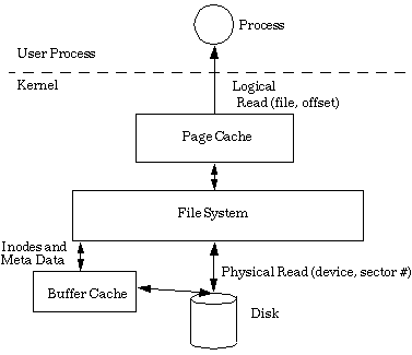
When we need to perform a sum() on this data, we can simply do a straightforward sequential read of the file. Though it won’t put all the data in memory, this scan will signal to the Linux kernel that the disk data is hot, and Linux will start caching.

To quote a kernel developer, “when you read a 100-megabyte file twice, once after the other, the second access will be quicker, because the file blocks come directly from the page cache in memory and do not have to be read from the hard disk again.” Flat files, for the win!

Of course, even if the whole file doesn’t fit into memory, we can still smartly load large chunks, and know exactly what document range our field values correspond to, thanks to the strict order. This can let us re-use the Bitsets from the earlier section to filter these subsets appropriately.

Lucene: Nice index, OK database

Lucene is not a database — as I mentioned earlier, it’s just a Java library. It’s coming from the world of information retrieval, which cares about finding and describing data, not the world of database management, which cares about keeping it.

That said, Lucene is an excellent building block for high-performance indices of your data. Solr and Elasticsearch are essentially wrappers on Lucene that use its good parts for information retrieval, and then try to build their own layer atop for persistence. Solr takes advantage of Lucene’s built-in “field storage” for this, while Elasticsearch stores JSON blobs inside a Lucene field, called “_source”.

Lucene goes even deeper than that, though: using Lucene’s API, you can build your own index format (see its Codecs API). Since Lucene’s data model is so flexible, when you squint, systems built with Lucene often look like “NoSQL” databases themselves.

With the rise of NoSQL, I’ve noticed another trend: NIH. No, no, not that NIH — I’m talking about Not Indexed Here. The rise of MongoDB and Cassandra has also led developers to “roll their own index”, mainly out of necessity.

For example, Cassandra encourages you to “determine exactly what queries you need to support”, and then store your data in a way to support those queries. Cassandra only really has one index — the partition index. So, you have to map all your problems into that one query pattern. Bummer.

Before MongoDB added full text search to its core, it encouraged developers to “use keywords stored in an array in the same document as the text field”. Same deal. An indexed keyword array lets you leverage MongoDB’s one-trick pony, the BTree index. What’s worse, the actual implementation of their built-in full-text search support doesn’t introduce any new indexing techniques. It just takes care of generating that keywords array for you, and then stuffing it in the BTree.

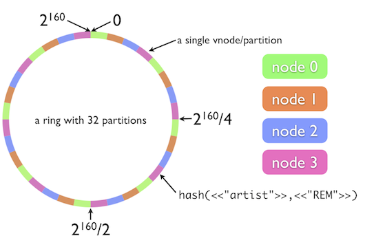
OK, I get it — every distributed database has to re-invent its approach to a consistent hash ring for your data. But, do they have to re-invent indexing, too?

In both of these cases, and in many others, you’d be better off using a Lucene index on your data. Invert your thinking, invert your index. Store your data where you wish, but then build a corpus of Lucene documents with fields corresponding to the data you actually need to find. Anything you put in a field will be indexed and queryable in ad-hoc ways. You just need to come to terms with your terms. But, as we’ve learned, anything can be a term. Convert those into a vocabulary you can actually understand. Then defy comprehension by converting it all into compressed Bitsets. Impress your friends once more by uninverting your inversion. When your sysadmin complains of memory usage, reveal that you’ve rebuilt the fancy database using none other than flat files. Marvel at how well your OS optimizes for them.

Then, query your Lucene index with pride — a decade-old technology, built on a century of computer science research, and a millennium of monk-like wisdom.

In other words, cutting-edge stuff.

Interested in Lucene, next-generation databases, and storing lots of data at scale? Especially if you’re a Python programmer who likes remote teams, you should look at Parse.ly — we’re hiring!

Thank you to Sal Gionfriddo, Didier Deshommes, and Otis Gospodnetić for reviewing an earlier draft of this post.